Data Compression

Source Coding¶

Shannon's Source Coding, 信源編碼、符號源編碼
information mapping (bits, characters, ....)

Entropy¶

Self-Information¶

by three assumptions
1. $I (p) \geq 0$
2. $I (p_{1} \cdot p_{2}) = I (p_{1}) + I (p_{2})$
3. $I (p)$ is continuous to $p$

thus, gives $I (p) = - \log (p)$

proof at p.25

Entropy¶

Given,

\begin{matrix} S = {s_{i} | p (s_{i}) = p_{i}} \end{matrix}

then,

\begin{matrix} H_{r} (S) = \sum p_{i} I (s_{i}) = \sum - p_{i} \log_{r} (p_{i}) \end{matrix}

note that $r$ is the base of log

Gibbs' Inequality¶

\begin{matrix} \sum - p_{i} \log (p_{i}) \leq \sum - p_{i} \log (q_{i}) \end{matrix}

the lower bound of cross entropy of $q_{i}$ and $p_{i}$ are $H (p_{i})$ .

Unique Decodable & Instantaneous Code¶

p32

Unique Decodable¶

not unique decodable example

\begin{matrix} (s_{1}, s_{2}, s_{3}, s_{4}) = (0, 01, 11, 00) \end{matrix}

then for the message $0011$ could be decoded as

0011 = {\begin{aligned} s_{4} s_{3} \\ s_{1} s_{1} s_{3} \end{aligned}

Instantaneous Code¶

instantaneous iff 沒有一個符號是另一個符號的字首
instantaneous ⇒ unique
the lengths of codes have to follow Kraft Inequality

Kraft Inequality¶

If instantaneous, then the code have to end at leaves.
thus, considering binary case only first we cannot build a binary tree for many short path(short coding length).
Therefore, in order to build an binary tree, we must follow

\begin{matrix} \sum \frac{1}{2^{L_{i}}} \leq 1 \end{matrix}

intuitive thinking – Considering taking a branch of binary tree have prob. 0.5 and 0.5, then the summation of prob. of all leaves is $1$ .
intuitively, the lowest bound of average lengths of codes is its entropy. (proof at p36.)

\begin{matrix} H_{r} (S) \leq L_{a v g} \end{matrix}

Shannon-Fano Coding¶

Since we know the lower bound of coding length is its entropy, then we can have the coding length (known as Shannon-Fano Length) as

\begin{matrix} - \log (p_{i}) \leq ℓ_{i} < - \log (p_{i}) + 1 \\ ⟺ ℓ_{i} = ⌈ - \log (p_{i}) ⌉ \end{matrix}

drawback example
Given $S = {s_{1}, s_{2}}$ , and $k$ is large

\begin{matrix} p_{1} = 2^{- k}, p_{2} = 1 - p_{1} \\ ⟹ l_{1} = k, l_{2} = 1 \end{matrix}

in Huffman coding, both $l_{1}, l_{2} = 1$ , but since $p_{1}$ is small when $k$ is large, this drawback isn't very critical.

Extension Code¶

quick concept – if we have an source code $S$ , then we can define an new source code $T = S^{n}$ (then the # of symbol in $T$ would be $| S |^{n}$ )
The $H (T) = n H (S)$ , and denote $L_{n}$ (average length of $n$ -order S.F. code), then

\begin{matrix} H (T) \leq L_{n} < H (T) + 1 \\ H (S) \leq \frac{L_{n}}{n} < H (S) + \frac{1}{n} \end{matrix}

thus when $n \to \infty$ , then $\frac{L_{n}}{n} \to H (S)$
aka Shannon's noiseless coding theorem.

Adaptive Huffman¶

start with one EOF and one ESC (always one in Huffman tree).
EOF – send when end of file.
ESC – send when new symbol is added to tree (send following with ascii of that symbol so that decoder can know what to decode).

JBIG & JBIG2¶

code for binary data directly ( $S \in {0, 1}$ )
JBIG – high order adaptive arithmetic (for $P (s_{t} | s_{(t - n) : (t - 1)})$ .
- since the target is binary, the high order coding table would be $2^{n}$ , much less than high order Huffman.
JBIG2 – Define decoding protocol only. That is the encoder side can be any algorithm, even lossy.

LZ¶

LZ77¶

sliding window and look-ahead buffer
find phrase in window, and encode text in look-ahead buffer
send (displacement, length, next_char)
in no match case, send (0, 0, next_char)
pros
- fast decode
cons
- slow encode
  - $O (n)$ , ( $n$ is windows size)
  - $O (m)$ , ( $m$ is look-ahead buffer size)
- worst case when no match
- prefer larger window size but cost too much
  - time efficiency ↓
  - compressed phrases size ↑
- loss memory (after dictionary is full of phrases, some of them have to be removed)

LZSS¶

improving version of LZ77
send $1$ bit indicating whether is no match instead of send (0, 0 next_char)
Circular queue with WINDOW_SIZE = $2^{n}$
Binary Search Tree for storing phrases (actually storing pointer to particular position of window).
- Node stores fixed-size length
- e.g. ("LZSS is better than LZ77") with fixed length $5$ , (search by comparing char-wise order)

graph TD
root(LZSS^)
l(^is^b)
ll(^bett)
lr(is^be)
r(ZSS^i)
rl(SS^is)
rr( )
rll(S^is^)
rlr(tter^)
root --- l
root --- r
l --- ll
l --- lr
r --- rl
r --- rr
rl --- rll
rl --- rlr

LZ78¶

create new phrase in dictionary at both encoder size and decoder size whenever no match
1. initially, there is only null string in dictionary.
2. thus whenever create a new phrase with length $n$ , there must exists a phrase with length $n - 1$ .
3. therefore, using multiway search tree to store phrases

graph TD
r('\0' <br> 0)
p1("'D' <br> 1")
p2("'A' <br> 2")
p3("'^' <br> 3")
p4("'A' <br> 4")
p5("'^' <br> 5")
p6("'D' <br> 6")
p7("'Y' <br> 7")
p8("'^' <br> 8")
p9("'O' <br> 9")

r --- p8
r --- p2
r --- p1
p1 --- p3
p1 --- p4
p1 --- p7
p4 --- p5
p4 --- p6
p6 --- p9

- in this case p1 = D, p3 = D^, p5=DA^, and so on...

example at p119
- thus encoder side only have to send phrase code (phrase id), without phrase's length.
  - i.e. (phrase_id, next_char)
cons
- slow decoding (have to maintain dictionary tree)

LZW¶

improving version LZ78
- defined every characters as phrases first, then send only (phrase_id, )
examples: PNG, ...

algorithm p122

encoder:

i := 0;
Dictionary phrases;
string in_buff;
in_buff.Add(str[i])

while
    in_buff.Add(str[++i])
    if in_buff not in phrases
        phrases.Add(in_buff)
        OUTPUT << phrases.IndexOf(in_buff.PopLast())
        in_buff := string(in_buff[-1])

decoder

i := 0
Dictionary phrases;
int in_buff;
string last_phrase

// init
INPUT >> in_buff
last_phrase := phrases[in_buff]
OUTPUT << last_phrase

while true
    INPUT >> in_buff
    OUTPUT << phrases[in_buff]
    phrases.Add(last_phrase + phrases[in_buff][0])
    last_phrase = phrase[in_buff]

Lossy¶

RMSE (Root Mean Square Error)
SNR (Signal-to-Noise Ratio)

$\begin{matrix} SNR = \frac{E [S^{2}]}{E [(X - μ)^{2}]} = \frac{E [S^{2}]}{σ_{r}^{2}} \\ {SNR}_{d B} = 10 \log_{10} SNR \end{matrix}$
- in 2d media case

\begin{matrix} SNR = \frac{Q^{2}}{σ_{r}^{2}} \end{matrix}

in which $Q = 255$ in 8-bits case.

DM¶

Delta Modulation
Adaptive DM (ADM)
- adaptive for the magnitude of $Δ$

DPCM¶

Differential Pulse Code Modulation

Predictor Optimization¶

objective

\begin{aligned} {\hat{x}}_{m}^{*} & = \arg min_{{\hat{x}}_{m}} σ_{e}^{2} \\ = \arg min_{{\hat{x}}_{m}} E [(x_{m} - {\hat{x}}_{m})^{2}] \end{aligned}

in which,

\begin{matrix} {\hat{x}}_{m} = \sum_{i \in [0, m)} α_{i} x_{i} \end{matrix}

then solve by differentiation, we have

\begin{matrix} E [(x_{m} - {\hat{x}}_{m}) x_{i}] = 0 \end{matrix}

thus

\begin{matrix} E [x_{m} x_{i}] = E [{\hat{x}}_{m} x_{i}] \\ R_{m i} = E [{\hat{x}}_{m} x_{i}] \end{matrix}

and further when $i = m$ ,

\begin{matrix} E [x_{m}^{2}] = E [{\hat{x}}_{m} x_{m}] \\ ⟹ σ_{e}^{2} = E [(x_{m} - {\hat{x}}_{m})^{2}] = \\ E [(x_{m} - {\hat{x}}_{m}) {\hat{x}}_{m}] = E [x_{m}^{2}] - E [{\hat{x}}_{m}^{2}] \\ ⟹ σ^{2} < E [x_{m}^{2}] \end{matrix}

p141

Quantizer Optimization¶

objective ( $N$ is number of order of quantizer)

\begin{matrix} D = \sum_{i \in [0, N)} \int_{d_{i}}^{d_{i + 1}} p (e) (e - r_{i})^{2} d e \end{matrix}

p143

Adaptive DPCM (ADPCM)¶

映射量化器
- $e = x_{m} - {\hat{x}}_{m}$
- $x_{m} \in [0, 2^{n})$ , thus normally $e \in (- 2^{n}, 2^{n})$
- however with known ${\hat{x}}_{m}$ , then $e \in [- {\hat{x}}_{m}, 2^{n} - {\hat{x}}_{m})$
替換量化器
- use multi quantizers, and encode with the best quantizer, and send which of quantizers.

Lossless DPCM¶

without quantizers, send the $e$ directly (or further using other lossless algorithm).
thus can be used as preprocessor for others like Huffman, Arith. (since quite popular).
more efficient then using adaptive like AHuff, AArith, but perform closely.

Non-Redundant Sample Coding¶

aka adaptive sampling coding

Polynomial Predictor¶

\begin{matrix} x_{t} = x_{t - 1} + Δ x_{t - 1} + Δ^{2} x_{t - 1} + \dots \end{matrix}

in which

\begin{matrix} Δ^{2} x_{t - 1} = Δ x_{t - 1} - Δ x_{t - 2} \end{matrix}

Polynomial Interpolator¶

1次內插法 = 扇形演算法 = SAPA2

AZTEC¶

p173
rules
1. use horizontal line if $\geq 3$ successive samples satisfy $x_{m a x} - x_{m i n} < λ$
2. otherwise, use slope. Further, if next sample have the same signed of slope and $| x_{m} - x_{m - 1} | > λ$ , then keep redundant.

CORNER¶

CORCER > SAPA2 > AZTEC
algorithm
1. 2-order diff, $x^{″} (i) = x (i + 1) + x (i - 1) - 2 x (i)$
2. $\forall i$ , if $x (i) > λ_{1}$ and $x^{″} (i)$ is local maximum, then make $x (i)$
3. then now have redundant samples $x (m_{1}), x (m_{2}), x (m_{3}), \dots$
4. for all redundant, find if $x (\frac{m_{1} + m_{2}}{2}) - \frac{x (m_{1}) + x (m_{2})}{2} > λ_{2}$ (that is, if the $x$ very concave (凹))
5. if not, add $x (\frac{m_{1} + m_{2}}{2})$ , as $x (m_{1_2})$ , and do ${x (m_{1})$ , $x (m_{1_2})}$ and ${x (m_{1_2}), x (m_{2})}$ as step 4.
6. if step4. so, continue

BTC¶

-Block Truncation Coding

Moment-Preserving Quantizer¶

target – find quantizer that make 1st and 2nd moment unchanged, and since

$\begin{matrix} σ^{2} = E [X^{2}] - E [X]^{2} \end{matrix}$

the variance $σ^{2}$ would also unchanged.
solution – Given $X_{t h}$ as the threshold (normally, mean of all pixels), and $q$ is # of $b$ cases

{\hat{x}}_{i} = {\begin{cases} a & if x_{i} < X_{t h} \\ b & otherwise \end{cases}

\begin{aligned} E [X] & = \frac{(m - q) \cdot b + q \cdot a}{m} \\ E [X^{2}] & = \frac{(m - q) \cdot b^{2} + q \cdot a^{2}}{m} \end{aligned}

then,

\begin{aligned} a & = E [X] - σ \sqrt{\frac{q}{m - q}} \\ a & = E [X] + σ \sqrt{\frac{m - q}{q}} \end{aligned}

solution2 (Absolute Moment BTC, AMBTC)
- since the square root is hard to compute, thus we maintain the absolute moment instead of 2nd moment.
$\begin{matrix} α = E [| X_{i} - μ |] \end{matrix}$

then, we can have,

$\begin{aligned} a & = E [X] - \frac{m α}{2 (m - q)} \\ b & = E [X] + \frac{m α}{2 q} \end{aligned}$

Transform Coding¶

Rotation Matrix

M (θ) = [\begin{matrix} \cos θ & - \sin θ \\ \sin θ & \cos θ \end{matrix}]

### Zonal Sampling - 區域取樣 1. 保留低頻，高頻通常小，不留 2. 低頻用比較多 bits 3. 固定 bits per block 但讓 variance 大(對其他 blocks 的同位置)的係數有比較多 bits - cons - 可能有很大難以忽略的係數

Threshold Sampling¶

臨界取樣
1. 設 threshold ，以下為 0，以上送位置與值

JPEG encode¶

get $F^{*} (u, v)$
scan with z order
First coefficient(DC) encode with DPCM and Huffman.
encode remains coefficients(AC) with the following law
1. omit $0$
2. lookup category $k$ at p220
3. according to category $k$ and # of $0$ before this coefficient, lookup table in p224.
4. append $k$ bits which indicates the index of AC coefficient in that category.

DCT¶

p209

Vector Quantization¶

Cost of encoding $O (n N_{c})$ , where $n$ is dimension of vector, $N_{c}$ is number of codebooks.
need memory $n N_{c}$

LBG¶

LBG演算法是由Linde,Buzo,Gray三人在1980年提出的。其算法與K-means雷同，根據當前劃分之群集計算誤差量，不斷調整映射區間(Mapping Region)及量化向量之量化點:

給定訓練樣本以及誤差閾值
訂定初始碼向量
將疊代計數器歸零
計算總誤差值，若不為第一次，則檢查與前一次誤差值差距是否小於閾值。
根據每一個訓練樣本與碼向量的距離d，找其最小值，定義為映射函數Q
更新碼向量：將對應到同一個碼向量的全數訓練樣本做平均以更新碼向量。

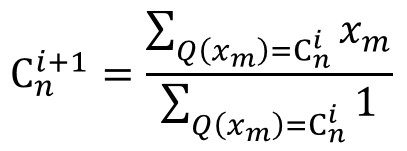
i為疊代計數器，C為該群集之代表，x為資料點，Q(x)為x量化後之群集代表C

疊代計數器加一
會到步驟四，直至誤差值小於閥值

LBG演算法十分依賴起始編碼簿，產生起始編碼簿的方法有以下幾種：

Tree-Structured Codebooks¶

$m$ -ways tree
Cost now decrease to $O (n \cdot m \log_{m} N_{c})$
Memory increase to $n m \frac{N_{c} - 1}{m - 1}$
- Because there are $N_{n} = (m + m^{2} + m^{3} + \dots)$ nodes,
  and that $N_{n} = m \frac{m^{\log_{m} N_{c}} - 1}{m - 1} = m \frac{N_{c} - 1}{m - 1}$
cons
- perform worse then full-search, since taking branch.

Product Code¶

use codebook represent vector direction with size $N_{1}$ , and codebooks represent vector length with size $N_{2}$ .
- this case, we can represent $N_{1} N_{2}$ vectors with only size $N_{1} + N_{2}$
  - therefore, in same time complexity and bit rate, perform better the full-search

M/RVQ¶

平均/餘值 VQ
1. 對每個 blocks (e.g. $n = 4 \times 4 = 16$ ) 減去平均
2. 傳送平均 (with DPCM or something)
3. do VQ and send

I/RVQ¶

內插/餘值 VQ
1. do subsampling to original image (assume $N \times N$ ) and would get sub-image ( $N / ℓ \times N / ℓ$ , normally $ℓ = 8$ ).
2. do up-sampling by interpolation, and get the residual image.
3. split residual image to blocks and do VQ.
pros
- perform better (less blocking artifacts) than M/RVQ.

G/SVQ¶

Gain/Shape VQ
- find and send the vector that match the most (has greatest dot product value)

CVQ¶

Classification VQ
1. split the image to blocks
2. classify blocks to categories
3. for every categories, there are some specific codebooks
normally use many small codebooks, but can reach similar performance with the normal VQ using large codebooks.

FSVQ¶

Finite State VQ
1. Given
  - codebooks per state $C (s_{i})$
  - transition function $s_{i} = f (s_{i - 1}, Y_{i - 1})$
2. given $s_{0}$ , and find $Y_{0}$ by $C (s_{0})$
3. get $s_{1} = f (s_{0}, Y_{0})$ , and find $Y_{1}$
4. until all done
cons
- one connection drop can cause serious consequence.